
Tutorial 02
|
Tutorial 02 |
Arithmetic |
|
Basic arithmetic operations in Excel |
|
 |
back to the terminology |
on to actions |
 |
Excel can be used as a simple calculator to perform simple arithmetic. For our second lesson we will use this fact to illustrate the many ways that Excel will help you in any laboratory course.
 With
any equation or formula, Excel requires that you first type an equal sign (=)
and then your equation. The equal sign tells Excel that the succeeding characters
constitute a formula. Following the equal sign are the elements to be calculated
(the operands), which are separated by calculation operators, such as the plus
sign or minus sign. For example, to add two numbers, say 3 and 2, you
would type into any empty cell the following: = 3 + 2 . The image to the right
shows this simple example entered into cell B2. Note the equation can be found
in both the formula bar and the cell B2.
With
any equation or formula, Excel requires that you first type an equal sign (=)
and then your equation. The equal sign tells Excel that the succeeding characters
constitute a formula. Following the equal sign are the elements to be calculated
(the operands), which are separated by calculation operators, such as the plus
sign or minus sign. For example, to add two numbers, say 3 and 2, you
would type into any empty cell the following: = 3 + 2 . The image to the right
shows this simple example entered into cell B2. Note the equation can be found
in both the formula bar and the cell B2.
 In order for Excel to perform the arithmetic, you must hit the <ENTER>
key. When this is done the answer, which is of course 5, appears in cell B2.
The image to the right shows the worksheet after the equation was entered. Note
the result is found in cell B2, but the equation is displayed in the formula
bar.
In order for Excel to perform the arithmetic, you must hit the <ENTER>
key. When this is done the answer, which is of course 5, appears in cell B2.
The image to the right shows the worksheet after the equation was entered. Note
the result is found in cell B2, but the equation is displayed in the formula
bar.
 Other basic arithmetic operations
Of course you can also use Excel to perform subtraction by substituting the plus sign (+) with the minus sign (-). Multiplication is performed with the asterisk (*) and division is performed using the forward slash (/). These equations are highlighted in cells C2:C5 in the image to the right. (You may be interested to know that equations can be printed to the screen by typing an apostrophe (') before the equal sign.)
Just as you learned in your math classes, formulas in Excel also calculate values in a specific order. Excel performs the operations from left to right, according to the order of operator precedence, starting with the equal sign (=). You can control the order of calculation by using parentheses to group operations that should be performed first. For example, in the example aboveto the, the highlighted cell C7 shows parentheses around the first part of the formula. This forces Excel to calculate the sum, 3+4, first and then divide the result by 2. Compare this to the equation in cell C8. Here there are no parentheses so the division, 4/2, is performed first then the addition is performed.
Another common operator that you will use quite often in your laboratory courses is the exponential operator. This is used, for instance, to square a number or take the cube root of another one. You use the caret (^) to perform exponential operations in Excel. Also note that the use of parentheses is often imperative when using the exponential operator. Below are some examples using the this common operator.
| Mathematical Expression |
Excel Expression |
Result |
 |
3^2 | 9 |
 |
3^(-2) | 0.11111 |
 |
8^(1/3) | 2 |
 |
100^(3/2) | 1000 |
For example, the image below shows how to use Excel to calculate  .
.
Click here to see a list of all the arithmetic operators used by Excel.
Of course we do not need a spread sheet application to add, subtract, multiply and divide; we all have calculators that do that. However, Excel is much more than a calculator. An Excel formula can also refer to other cells within the worksheet. For instance, in the example below, cells A2 and B2 display the length and width of a barley leaf. To determine the area of the leaf, we can use the formula Area = (length)(width). To do this in Excel follow these steps:
 Click
on cell C2, since this is the most logical place for the result to be displayed.
Click
on cell C2, since this is the most logical place for the result to be displayed.
In the above example, the cell that contains the formula (i.e., cell C2) is known as the dependent cell because its value depends on the values in cells A2 and B2. Whenever a cell that the formula refers to changes, the dependent cell also changes, by default. For example, if the value of the leafs length in the above example changes, the result of the formula =A2*B2 also changes. Try it and prove it to yourself! If you use constant values in the formula instead of references to the cells (for example, =30*5), the result changes only if you modify the formula yourself. You can type a formula once and use it thousands of times.
Microsoft Excel contains many predefined, or built-in, formulas, which are known as functions. Functions can be used to perform simple or complex calculations. Among the most frequently used functions are the SUM, AVERAGE and SQRT functions.
| To add a column or a row of numbers follow the steps below:
|
To average a column or a row of numbers follow the steps below:
|
| To find the square root of a number located within a worksheet cell follow the steps below:
|
|
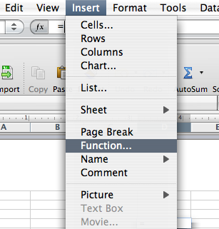
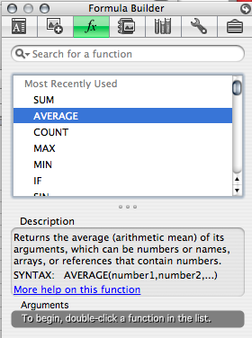
You can see the complete list of Excel's built-in mathematical and trigonometric
functions and their descriptions by selecting the Insert menu and selecting
Function... The Formula Builder window will be displayed. A description of each
function will appear as you point to it. Clicking on the function will add it
to the formula bar and bring up a dialog box to help you select the variables.
 |
|
 |
|
back to terminology |
 |
on to actions |
|
Copyright © 2000, St. Mary's College of Maryland. All Rights Reserved.
Please send comments, problems or request for topics to
Walter I. Hatch
wihatch@smcm.edu
August 11, 2005