
 |
Tutorial 03 |
Actions |
|
Basic data and text manipulation in Excel |
|
 |
back to arithmetic |
on to algebra |
 |
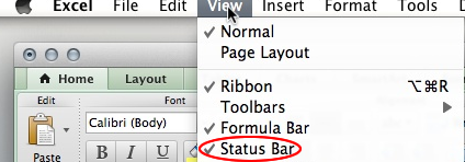
There are a few thing that you can do with every new spread sheet that will save time and prevent errors later. The first is to use the view menu to insure that you can see useful tools. On the menu bar select the view drop down menu and check Normal, Ribbon, Formula bar, and status bar. as Indicated here. This will insure that your spread sheet is not presented with the page brakes that would only be useful if the spreadsheet were to be printed on paper. It will also make ribbon visible. In addition it will insure that you can see (and type on) the formula bar allowing you to enter and edit formula easily. The status bar makes current view (Normal or Page Layout) visible at the bottom of the spread sheet.
These are not default settings and you you can avoid frustration by insuring that these set up actions are performed on each new sheet.
There are a few things you can do
to your worksheet that makes it more readable. This will greatly help your
keep track of your data and help your instructors ascertain where you are making
your mistakes. These formatting tools will also be required to produce figures
and tables that comply with the requirement of the Biology Department Style manual Here we discuss a few of the things you can do to improve
the look of your worksheet. All of these basic actions can be accessed from
Home ribbon as illustrated below.
 In
this tutorial we will take you through a mock experiment where we measure the
diameter of several spheres and then calculate the volume of those spheres. Go ahead and open a worksheet as described above. First enter the data as shown at the right.
As you can see, the data is there but much work is required to get the worksheet into an acceptable form. You should follow the steps on your own worksheet.
The data shown above has no heading. Your instructor can't possible know what the data represents and in a few days you wont know either. You first need to add column headings above the data telling the world what the numbers represent. A title for the data set would also be helpful.
Obviously there is no room for a heading so you must move the data to another location further down on the worksheet. You could retype the data, or copy and paste it three cells down or simply add 2 rows by highlighting the first two rows, right (control) clicking and selecting insert cells as shown. You should make a mental note to start your data entry on line 3 or 4 on the next sheet.

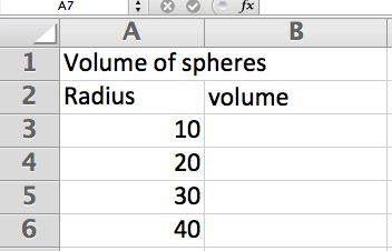 Now
we have space to add a title to our data table. Since we are determining
the volume of several spheres, let's entitle the data table "Volume
of Spheres". Put this title in cell A1. We also need column headings.
In cell A2 type "Radius" because the data below the heading are
the measurements of the radius. Let's also place a heading for the resulting
volume calculations. In cell B2, type "Volume". This is still not compliant with the style manual and the headings need to be centered. Click both the horizontal and vertical centering icon on the home ribbon and shown below.
You are now ready
to enter the formula that you will use to calculate the volume of the spheres.
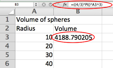 Enter Your Formula
 You should recall that the volume of a sphere is given by the formula ![]() ,
where r is the sphere's radius and p which can be entered as an Excel function (pi()). Therefore, the formula that you will use to find the volume of the first sphere
is =(4/3)*pi()*(A3^3). Enter this formula in cell B3. It will appear on the formula bar where it can be checked and edited. Be careful to define the order of mathematical operations with parenthesis The result
(4188.790205 cm3) is displayed in the cell.
,
where r is the sphere's radius and p which can be entered as an Excel function (pi()). Therefore, the formula that you will use to find the volume of the first sphere
is =(4/3)*pi()*(A3^3). Enter this formula in cell B3. It will appear on the formula bar where it can be checked and edited. Be careful to define the order of mathematical operations with parenthesis The result
(4188.790205 cm3) is displayed in the cell.
We could repeat this process for each radius in the table and type new formulas in each cell. However, a fastest way to determine the volume of the remaining spheres is to use the copy and paste functions. It would be useful to copy the formula in cell B3 and paste it to cell B4 through B6. An even faster (and more appropriate) way to accomplish this is to propagate the formula. Select the formula cell B3 and move the cursor to the lower right corner of the cell until it changes into a a small plus sign (+). Now simply drag the formula down to cells B4 through 6.
The formula is then moved to these destinations. Note that the pasted or propagated formula automatically changed the cell reference to use the appropriate radius in the calculation.
It is always a good idea to double-check the first and last cells with a calculator after a paste just to make sure the formulas were correct. I find it easier to simply substitute a test value that I already know the answer for and then undo the substitution once I know the formula is ok.
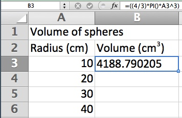 The
radius and volume column headings are missing the units for the data.
Is the radius 10 cm, 10 au, 10 in? Of course, units are need. The best way
to indicate units is place them in parentheses. Go ahead and add "(cm) to the heading in A2.
Notice the units of volume is cm3. Students commonly use the ^designation to indicate exponents. This is the proper way to indicate exponents in Excel formulae, but, it is not appropriate for table headings and it will cost you points. Instead of typing (cm^3), type (cm3), and select just the the 3. Now go to the menu bar and click on Format then Cells then Font and then check the superscript box. The 3 become super scripted as shown to the right. This is not optional; you will use credit if any of your heading do not use appropriate super and sub scripting.
![]()
![]() If you have read the style manual, you realize that headings should be centered. Centering is easily accomplished by selecting the cells containing the headings and then
selecting the centering icons (verticaland horizontal) under the alignment section of the home ribbon.
If you have read the style manual, you realize that headings should be centered. Centering is easily accomplished by selecting the cells containing the headings and then
selecting the centering icons (verticaland horizontal) under the alignment section of the home ribbon.
Notice that this produces the undesirable results shown in A below. The table title is centered only in column A.
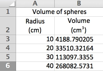
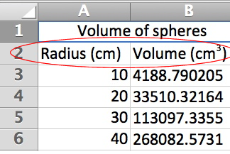
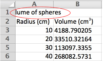 To fix this, simply select both cells A1 and A2 and merge them together to center the table title over the entire table as shown in B . The merge controlis located to the right of the centering controls indicated above.
![]() Show at B to the right
Show at B to the right
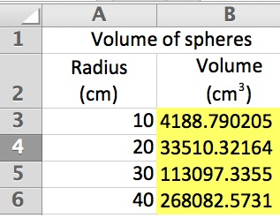
Notice that after the centering, the column headings are now crowded and difficult to read. To keep the heading and the unit in the same cell with out extending the width of the column, select Wrap Text from the Home ribbon. Now you can simply add spaces in front of the until they jump to the second line. Inconvenient? Yes, but Microsoft eliminated the shift enter soft carriage return we were all used to. Resulting in C to the right.
 To
really draw attention to the most important results of the experiment, you
can shade or color-in the cells containing formulas and final results.
This is customarily used to indicate any cells that contain the results of a calculations and is required on worksheets that are submitted for evaluation.
To do so highlight (select) the cell or cells you want shaded, Then on the home ribbon click the fill icon, ![]() ,
and select the desired color. Pale yellow is traditional.
,
and select the desired color. Pale yellow is traditional.
Note: This would be inappropriate for a table in a formal lab report but it makes it easier for others to read your spreadsheets and faster for you to navigating your your own spreadsheets.
It
is may be helpful to emphasize text like titles, column headings, and final results.
One way to make text stand out is to make it bold. To make the entire
contents of a cell bold, for instance the title found in cell A1, simply highlight
(select) the cell (or cells) and click the Bold Button, ![]() ,
on the Home ribbon. You
need not make the entire cell contents bold as shown above. For instance, you
can make the heading bold while the units are displayed as normal text. To
do this, on the formula bar, highlight the text you wish to make bold
and then click the Bold Button,
,
on the Home ribbon. You
need not make the entire cell contents bold as shown above. For instance, you
can make the heading bold while the units are displayed as normal text. To
do this, on the formula bar, highlight the text you wish to make bold
and then click the Bold Button, ![]() ,
on the Home ribbon
,
on the Home ribbon
 Any
good Biology laboratory student knows that 2.2 times 5.1 is 11, not 11.22 like
your calculator says. This is, of course, due to the number of significant
figures used. The numbers 2.2 and 5.1 both have two significant figures,
therefore, the answer must also have two significant figures. By default Excel
displays the maximum number of decimal places. However, the number of decimals
displayed can be manually forced by using the Increase Decimal Button, and
Decrease Decimal Button,
 ![]() ,
depending on the situation.
,
depending on the situation.
Note:
Older versions required the cell to be formatted as "number" for the decimal adjustments to function. Now simply clicking one of the
![]() buttons automatically formats the cell as numbers and adjusts the number of decimal places.
buttons automatically formats the cell as numbers and adjusts the number of decimal places.
Note: Adjusting the significant figures for whole numbers is accomplished by using the =Roundup and = Round down functions. For example
=ROUNDUP(31415.92654,-2) Rounds 31415.92654 up to 2 decimal places to the left of the decimal (31500). The -2 argument tells excel to round the numbers to the right of the decimal. If you are would like a more indepth discussion, click here to get to the MSExcel help file on rounding in MSExcell
 We
are almost done making your worksheet presentable. If you worksheet
looks a little cramped. Resize the columns so the data and results
are a little more readable. To do that, click the boundary on the right side
of any column heading (A,B,C etc) and drag it to the appropriate width.
 If want several columns to be the same width, you
can resize a number of columns at once by selecting the columns you want to
change, and then drag a boundary to the right of a selected column heading.
Each highlighted cell will automatically become resized. The same technique can also be used on worksheet row height .
 Note: If the width of a cell is too small, the cell contents will not be able
to be displayed properly. Its appearance will be determined by the alignment setting,
 ![]() , on the the Home ribbon and it might appear truncated or continued in the next cell. Numbers behave differently, and the ###### error will appear in the cell. To fix the problem,
simply increase the width of the cell.
, on the the Home ribbon and it might appear truncated or continued in the next cell. Numbers behave differently, and the ###### error will appear in the cell. To fix the problem,
simply increase the width of the cell.
![]() You
can also change the font style and font size to make certain
text, like titles and headings, more noticeable or to match the font to be used in your MSWord document.
You
can also change the font style and font size to make certain
text, like titles and headings, more noticeable or to match the font to be used in your MSWord document.
By default, all text is left-aligned in a cell. To change the alignment,
select the desired cell (or cells) and then click on one of the alignment buttons,
![]() to adjust the horizontal alignments or the
to adjust the horizontal alignments or the
![]() to adjust the vertical alignment
to adjust the vertical alignment
 When
including your tables in formal lab reports you must add borders to
the cells to make them compatible with the Biology Department Style manual The easiest way to add borders
to a cell or cells, is to highlight the desired cells, click on the Borders
Drop down Button,
 ![]() ,
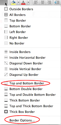
on the Home ribbon and then select the appropriate border from the drop down list. Unfortunately the border that you need to comply is not necessarily on the default list and you may need to select Border options
,
on the Home ribbon and then select the appropriate border from the drop down list. Unfortunately the border that you need to comply is not necessarily on the default list and you may need to select Border options
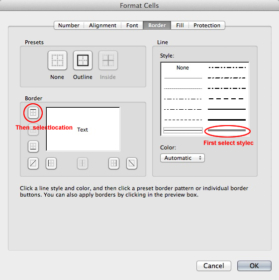
I recommend starting with the double line border required required at the top of the table. Select the top cell (merged A1 B1) and click the add borders icon ![]() on the Home ribbon. The border you need is not shown so would need to build it. Selecting border options from the list of border formats. This will open the dialog shown to the right. Now select the double line from the styles then select top border from the position list. Click ok and your table should have a double tine at the top.
on the Home ribbon. The border you need is not shown so would need to build it. Selecting border options from the list of border formats. This will open the dialog shown to the right. Now select the double line from the styles then select top border from the position list. Click ok and your table should have a double tine at the top.
The single line above and below the data are much easier. Select all if the data (A3:B6) and again click
the borders icon ![]() on the Home ribbon. This time you will find top and bottom border as one of the options click it and your done. It is difficult to see your borders if tour table starts in cell A1 but if you add a line above and a column to the right you borders will show nicely.
on the Home ribbon. This time you will find top and bottom border as one of the options click it and your done. It is difficult to see your borders if tour table starts in cell A1 but if you add a line above and a column to the right you borders will show nicely.
Reminder:
tables for inclusion in a lab report must be formatted according to The Biology Department Style manual
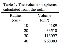 Formal
tables for inclusion in lab reports created in word processor programs like
MS Word must conform to the table styles discussed in the Biology Department Style manualas shown here. You will find that the
creation and formatting of the table are best accomplished within Excel prior
to pasting
them into MS Word. Check to be certain
that you have a table number, descriptive title, column headings and appropriate
grid lines (and no others) before you proceed. Here the the table number has been added instead of the title and the font has been changed to match the word document.
Moving your table to MSWord
Note: This is now a simple text table and changed data will not be reflected in calculations. If you modify the spread sheet you will need to copy/paste again. It is possible to paste a "live" Excel table that will allow recalculations and other Excel modifications by selecting Paste special and Paste as a Microsoft Excel work sheet object but I recommend reserving that option until you have considerable experience with MSWord
Worksheets submitted for grading:
When submitting printed worksheets for evaluation,
it is important that you
both highlight calculated cells and print your formulas so your instructor can follow your steps
and and
help
you identify
errors. If you are submitting an electronic version, u\you should highlight calculation cells, but, it is not necessary to include the formuls as they are a part of the workbook and can be accesed electronically. You do, however, need to comply with the guide lines for electronic submission.
Tables and Graphs submitted for grading:
Paper submission: When submitting Tables and graphs
as part of a formal lab report they need to be exported to MSWord and then printed. Of course they must conform to the Biology Department Style manual. Check to be certain that required borders are in place.
Electronic submission: If electronic submissions are required, be certain that you conform to all of the filenaming conventions before submission.
Recomendation: Include table headings in a merged cell at the top of the table prior to expert. The cell should extends across the entire width of the table. This will insure that the table legend text extends across the entire table and does not extend beyond the width of the table.
Recommendation: For graphs to be exported to MSWord, do not include graph legends (Figure number and discription) on the excel chart prior to export. While this will produce a style manual compliatable figure your instructor can not annotate these legends electronically.
 |
back to arithmetic |
on to algebra |
 |
Copyright © 2000, St. Mary's College of Maryland. All Rights Reserved.
Please send comments, problems or request for topics to
Walter I. Hatch
wihatch@smcm.edu
January 14, 2012