 Laboratory
01Laboratory
01
Laboratory
01Laboratory
01By now you should all be aware of the basic phenomenon of osmosis and the problems it presents to living organisms. Remember that cells are bags of ionic and non ionic solutes surrounded by a semi permeable membrane. Cells will, therefore, behave like osmometers. Cells placed in a hypotonic medium will be faced with an influx of water while cells in a hypertonic medium will lose water to the external environment. Organisms must have mechanisms to deal with the osmotic problem or remain restricted to environments that are isoosmotic to their internal environments. These mechanisms can include morphological adaptations such as cell walls that physically contain the pressure and prevent osmotic damage to cell membranes. Physiological mechanisms include active regulation of the osmotic concentration of body fluids by pumping ions and moving water or passive conformation of body fluids to the osmotic concentration of the environment. Some animals have developed behavioral mechanisms as well, allowing them to migrate to more favorable conditions or seal themselves off from adverse osmotic conditions.
If we can easily ascertain the osmotic concentration of environmental and organismal fluids, certain fundamental questions can be asked of a wide variety of aquatic and terrestrial organisms. What is the impact of desiccation on blood or hemolymph osmotic pressures in organisms exposed to varying degrees of stress? Or, how do organisms respond in terms of osmotic homeostasis when confronted with an increasing or decreasing salinity? It is your goal to determine the effect of varying environmental salinities on the osmotic concentration of three groups of euryhalinic organisms and to draw conclusions as to their mechanisms of adapting to these salinity changes.
Osmotic concentration or osmolality (Osm) is, by definition, an expression of the total number of solute particles dissolved in one kilogram of solvent without regard for particle size, density, configuration, or electrical charge. Osmotic pressure and water potential are related to osmotic concentration as well as temperature and pressure. It would be very tedious to determine osmotic conditions by describing the concentrations of all of the various inorganic and organic constituents in the external and internal environment of an organism. Therefore, osmotic concentrations are usually expressed as the equivalent concentration of an ideal nonelectrolyte and this is determined indirectly from one of the colligative properties of a solution.
Vapor pressure and freezing point are among the colligative properties of solutions. When compared with pure solvent, these properties are altered in proportion to the number of solute particles dissolved in each kilogram of solvent (water in the case of biological solutions). Thus, a measurement of either property affords an indirect means of determining solution concentration, or osmolality, independent of solute species. Changes in the freezing point and vapor pressure of solutions are the basis for all contemporary laboratory osmometers. The osmotic concentration of small volumes of biological fluids such as blood plasma, coelomic fluid, and urine can be quickly and accurately determined by means of either of these techniques, although vapor pressure methods have certain advantages.
The merits of the vapor pressure method stem from the fact that it does not require an alteration in the physical state of the specimen. Concomitant advantages include:
In vapor pressure osmometry the specimen is pipetted onto a solute-free paper disc in a circular sample holder. The sample holder is then conveyed into the instrument by means of a slide and locked in place. Locking initiates the automatic measurement sequence. The sensing element is a fine-wire thermocouple hygrometer. It is suspended in a unique, all-metal mount which, when coupled with the sample holder, forms a small chamber enclosing the specimen. Vapor pressure soon rises to equilibrium in the chamber airspace.
The ambient temperature of the air, sensed by the thermocouple, becomes the reference point for the measurement. Under micro-processor control, the thermocouple then seeks the dew point temperature within the enclosed space, giving an output proportional to the differential in temperature. The difference between the ambient temperature and the dew point temperature is the dew point temperature depression. - Dew point depression like the other collagist properties of water is directly related to osmolarity. The sample chamber is maintained at a normal temperature of 37°C. Dew point temperature depression is measured with a resolution of 0.00031 °C.
Osmolality is an expression of the total concentration of dissolved particles
in a solution without regard for particle size, density, configuration, or
electrical charge. Indirect means for the measurement of osmolality are afforded
by the fact that the addition of solute particles
to a solvent changes the free energy of the solvent molecules. This results
in a modification of the cardinal properties of the solvent, i.e., vapor pressure,
freezing point, and boiling point. Compared with pure solvent, the vapor pressure
and freezing point of a solution are lowered, while its boiling point is elevated,
provide that a single solvent is present in the solution. Solutions containing
more than one solvent generally behave in more complex ways. In single-solvent
solutions, the relative changes in solution properties are linearly related
to the number of particles added to the solvent, although not necessarily linearly
related to the weight of solute, since solute molecules may dissociate into
two or more ionic components. Since these properties all change linearly in
proportion to the concentration of solute particles, they are known as "colligative"
properties.
Osmotic pressure is also a colligative property of a solution, but unlike the other three, it is not a cardinal property of the solvent. Solution osmotic pressure can be measured directly using a semipermeable membrane apparatus, but only with respect to those solute particles that are impermeable, since smaller solute particles freely diffuse across the membrane and do not directly contribute to osmotic pressure. Such a measurement is referred to as "colloid osmotic pressure" or "oncotic pressure." It is expressed in terms of pressure, in mmHg or kPa. Total osmotic pressure, i.e., that which a only be made indirectly by comparing one of the solution colligative properties with the corresponding cardinal property of the pure solvent. The first practical laboratory instruments developed for routine measurement of osmolality were based upon depression of the freezing point and, until recent years, all osmometers for large-scale testing were based upon this methodology.
The
Vapro osmometer embodies newer technology. It is based upon a measurement
of vapor pressure depression made possible by
thermocouple hygrometry. The vapor pressure method enjoys a significant intrinsic
advantage over the measurement of either freezing
point depression or boiling point elevation in that it can be performed without
the necessity for a change in the physical state of
the specimen. It is thus a passive technique of measurement that is free from
measurement artifacts that often occur when the specimen to be tested must
be altered physically. This fundamental difference in methodology gives rise
to the many advantages of the vapor pressure osmometer over the older method.
In the Vapro vapor pressure osmometer, a 10 microliter sample of the solution
to be tested is pipetted onto a small, solute-free paper
disc which is then inserted into a sample chamber and sealed. A thermocouple
hygrometer is incorporated integrally within the chamber. This sensitive temperature
sensor operates on the basis of a unique thermal energy balancing principle
to measure the dew point temperature depression within the chamber. This parameter,
in itself a colligative property of the solution, is an explicit function of
solution vapor pressure.
The sample is introduced into the chamber and the chamber is closed. Simultaneously, “In Process” and a countdown by seconds is displayed. (This remains until the end of sequence at Program Step 4.) At this point, there will generally be some difference between the temperature of the specimen and the temperature of the sample chamber. Temperature equilibrium occurs within a few seconds. The vapor pressure may also reach equilibrium during this interval. The microvoltmeter reads the amplifier voltage to establish the reference for the measurement.
An electrical current is passed through the thermocouple, cooling
it by means of the Peltier Effect to a temperature below the dew point. Water
condenses
from the air in the chamber to form microscopic droplets upon the surface of
the thermocouple.
Electronic circuitry “pumps” thermal energy from
the thermocouple via Peltier cooling in such a way as to cancel out heat influx
to the thermocouple by conduction,
convection, and radiation. Given this, the temperature of the thermocouple
is controlled exclusively by the water condensing upon its surface. Thermocouple
temperature, depressed below the dew point in Step 2, rises asymptotically
toward
the dew point as water continues to condense. When the temperature of the thermocouple
reaches the dew point, condensation ceases, causing the thermocouple temperature
to stabilize.
The reading on the display is proportional to the vapor pressure of the solution.
When this final reading is reached, a chime sounds and the “In Process” changes
to “Osmolality”. The result is displayed in Sl units of osmolality—mmol/kg.
ation by a preamplifier, the signal is processed by the microprocessor
to provide calibrate and compensate functions and display the reading.
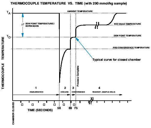 The graph on the right is a plot of thermocouple temperature versus time as
the instrument cycles through the program, beginning with chamber closure (time
= 0). The graph depicts the excursion of thermocouple temperature that typically
occurs during each of the program steps outlined above. TA is the ambient temperature
in the chamber. TD is the dew point temperature, and ∆T is the dew point temperature
depression. The output is proportional to ∆T. Assuming that the chamber remains
closed while the osmometer displays the final reading at Step 4, the thermocouple
temperature returns to TA after holding at the wet bulb depression temperature
until all of the water has evaporated from the thermocouple. If the chamber
is opened, the water will evaporate almost instantly and the thermocouple temperature
will quickly return to ambient.
The graph on the right is a plot of thermocouple temperature versus time as
the instrument cycles through the program, beginning with chamber closure (time
= 0). The graph depicts the excursion of thermocouple temperature that typically
occurs during each of the program steps outlined above. TA is the ambient temperature
in the chamber. TD is the dew point temperature, and ∆T is the dew point temperature
depression. The output is proportional to ∆T. Assuming that the chamber remains
closed while the osmometer displays the final reading at Step 4, the thermocouple
temperature returns to TA after holding at the wet bulb depression temperature
until all of the water has evaporated from the thermocouple. If the chamber
is opened, the water will evaporate almost instantly and the thermocouple temperature
will quickly return to ambient.
The relationship between sample osmolality and the reading obtained by the
osmometer is governed by fundamental considerations. Vapor pressure depression,
a linear function of osmolality, has been identified as one of the colligative
properties of a solution. The relationship between vapor pressure depression
and dew point temperature depression is given by ∆T = ∆e/S where ∆T is the
dew point temperature depression in degrees Celsius, ∆e is the difference between
saturation and chamber vapor pressure and S is the slope of the vapor pressure
temperature function at ambient temperature. The Claussius-Clapeyron equation
gives S as a function of temperature (T), saturation vapor pressure (eo,) and
latent heat of vaporization (£f): eo£f S = RT2 where R is the universal gas
constant. The dew point temperature depression, ∆T, is measured as a voltage
signal from the thermocouple. This voltage is equal to ∆T multiplied by the
thermocouple responsivity which is approximately 62 microvolts per degree Celsius.
After voltage amplification by a preamplifier, the signal is processed by the microprocessor
to provide calibrate and compensate functions and display the reading.
In our instrument a microprocessor controls the measurement cycle, which requires 58 seconds for samples having osmolality of 200 mmol/kg or higher. If the osmolality of the specimen is below 200 mmol/kg, a manual selection extends the measurement time to 88 seconds and improves the accuracy of the reading.
Traditionally, osmolality has been expressed as milliosmoles per kilogram, with various abbreviations such as mOs/kg, mOsm/kg, and mOsmol/kg. The inclusion of the letters Os was intended to emphasize that osmolality is defined as the concentration, expressed on a molal basis, of the osmotically active particles in true solution. Thus, one mole of sodium chloride dissolved in a kilogram of water (1 mol NaCl/kg) would have an ideal osmolality of 2 Osm/kg, since a molecule of sodium chloride dissociates in solution to produce two ions, that is, two osmotically active particles.
With complex solutions, such as blood and other biological fluids, analytical variables are universally expressed as the concentration of specific ions and of undissociated solute particles. It follows that a molal solution of NaCl can be analytically expressed as a combination of a molal solution of sodium ions and a molal solution of chloride ions. The total concentration of solute particles (the osmolality) is therefore 2 molal. Hence the osmolality can be expressed simply as 2 mol/kg without the necessity of introducing the "osmole" concept.
It must be emphasized that this example assumes ideal conditions for the sake of clarity. In fact, a molal solution of sodium chloride will have an osmolality value slightly less than 2 mol/kg because the residual mutual attraction of the hydrated ions reduces their mutual independence by a factor called the osmotic coefficient. Since the coefficient varies with the solute concentration, the relation between osmalality and concentration of solute is not linear. For this reason, measurements of osmolality made on laboratory-diluted specimens, with subsequent multiplication by the dilution factor, will not give valid results and can only be considered estimates.
The Commission on Clinical Chemistry of the International Union of Pure and Applied Chemistry (UPAC) and the International Federation of Clinical Chemistry (IFCC) have recommended that the unit of osmolality be mmol/kg, and this has been adopted by the journal "Clinical Chemistry" as part of its general acceptance of Standard International (S.I.) units. If it's good enough for the Commission it's good enough for your lab report.
Read through the instructions and prepare a step-by-step protocol that will eliminate wasted time, i.e. if your blood requires centrifugation start that first so that other chores can be accomplished during the spin.
Observe the labels on the crab condominiums in the SH wet lab and place in in each experimental salinity at least 48 hours prior to the experiment. Each replicate will require:
If each team gets a sample from each organism we will have six replicates. Or you may work as a super team with each lab team sampling only one type of organism. Either way remember your report won't be convincing with out statistical analysis so think about how many replicates you will need.
The pugnacious nature and cannibalistic tendencies of the blue crab requires some special precautions if they are to be maintained in close quarters. Any method of preventing the use of their chelipeds will work, but the removal of the cheliped is your best insurance. The decapod crustacea have the ability to automize limbs if their retention would threaten the safety of the organism. You need only threaten the crab by holding the cheliped in a Bunsen burner flame and the distressed crab will contract specialized muscles that will drop the claw and seal off the circulatory system. Failure to disable or remove the chelipeds will threaten the success of everyone's experiment. It is not necessary or advisable to disarm fiddlers.
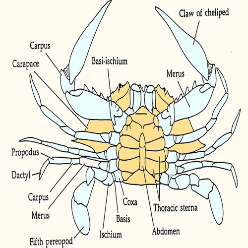 Collect
at least (250 ul) (1/4 microfuge tube) of
blood by piercing the membrane between fifth
periopod and body with a 3 ml syringe and 16-18 gauge needle. Transfer
the blood immediately to a micro centrifuge tube and stir it vigorously
to promote clotting prior to centrifuging. Alternatively, swiftly cut through
the coxa of the fifth periopod and collect the blood from stump directly
into a 1500ml microfuge tube.
If you utilize this technique, it is critical to avoid contamination
of your sample with water draining from the branchial chamber by wrapping
the animal in a paper towel. Stir the blood vigorously to promote clotting
prior to centrifuging. Smaller animals will require modification of
this technique. Fiddlers are best sampled by cutting basi-ischium of
the large cheliped of males and then pumping the dactyl to express the
blood. Shrimp will not provide much blood. cutting through the abdomen
just posterior to the heart and collecting blood directly into hematocrit
tubes should work.
Collect
at least (250 ul) (1/4 microfuge tube) of
blood by piercing the membrane between fifth
periopod and body with a 3 ml syringe and 16-18 gauge needle. Transfer
the blood immediately to a micro centrifuge tube and stir it vigorously
to promote clotting prior to centrifuging. Alternatively, swiftly cut through
the coxa of the fifth periopod and collect the blood from stump directly
into a 1500ml microfuge tube.
If you utilize this technique, it is critical to avoid contamination
of your sample with water draining from the branchial chamber by wrapping
the animal in a paper towel. Stir the blood vigorously to promote clotting
prior to centrifuging. Smaller animals will require modification of
this technique. Fiddlers are best sampled by cutting basi-ischium of
the large cheliped of males and then pumping the dactyl to express the
blood. Shrimp will not provide much blood. cutting through the abdomen
just posterior to the heart and collecting blood directly into hematocrit
tubes should work.
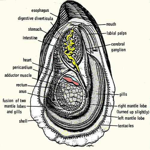 Collect
blood by carefully open the oyster and reflect the mantle away from
the dorsal body wall. The heart
should be visible, beating within the pericardial cavity. Drain the
mantel cavity and blot the pericardium dry with tissue and carefully
pierce the membrane with fine tipped forceps, reflect the membrane and
collect as much blood as possible (at least 250 ul) with a narrow bore
disposable pipette. Transfer the blood to a 1500 ml microfuge tubes.
If you damage the pericardial membrane while opening the oyster, you
can still collect an uncontaminated sample by shaking the all of the
fluid from the oyster and then waiting for thee pericardial cavity to
refill.
Collect
blood by carefully open the oyster and reflect the mantle away from
the dorsal body wall. The heart
should be visible, beating within the pericardial cavity. Drain the
mantel cavity and blot the pericardium dry with tissue and carefully
pierce the membrane with fine tipped forceps, reflect the membrane and
collect as much blood as possible (at least 250 ul) with a narrow bore
disposable pipette. Transfer the blood to a 1500 ml microfuge tubes.
If you damage the pericardial membrane while opening the oyster, you
can still collect an uncontaminated sample by shaking the all of the
fluid from the oyster and then waiting for thee pericardial cavity to
refill.
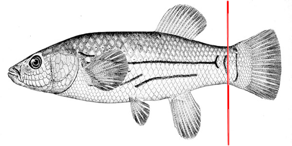 Unfortunately you can not kill the fish first as a beating heart is required
to pump the blood out of the aorta. MS-222(Tricaine methane-sulfonate)
is, however an efective fish anesthetic and you shoud immerse your fish in
a 100mg MS222/l of culture water. Immerse the fish for about 10 min prior
to collecting the blood and return them to a leathal solution of 250mg/l
when you have compleated the proceedure. Work as quickly and humanly as possible.
A pooled blood sample from three fish should be enough for both osmotic pressure
and ion concentration measurements.
Unfortunately you can not kill the fish first as a beating heart is required
to pump the blood out of the aorta. MS-222(Tricaine methane-sulfonate)
is, however an efective fish anesthetic and you shoud immerse your fish in
a 100mg MS222/l of culture water. Immerse the fish for about 10 min prior
to collecting the blood and return them to a leathal solution of 250mg/l
when you have compleated the proceedure. Work as quickly and humanly as possible.
A pooled blood sample from three fish should be enough for both osmotic pressure
and ion concentration measurements. Note: centrifuged samples can not stand on the pellet. Either use them right out of the centrifuge or decant thne supernate into fresh labeled tube.
All vertebrate blood samples must be centrifuged prior to osmometry or freezing as cellular disruption will liberate variable amounts of osmotically and ionically active material, affecting the results of this experiment as well as varying ionic concentrations that will alter the results of next week's experiment. Invertebrate blood will have significantly fewer cells, but if all samples are to be treated alike you should centrifuge them as well as your water samples.
For these relatively large samples you will use an Eppendorff microfuge. Make certain that the samples are in 1500 ml microfuge tubes and that the caps are tightly sealed. To insure that the rotor remains balanced, place the tubes in the microfuge such that each tube has a tube with equal volume directly across from it. The relatively low speed and low sample volume of the microfuge make it unnecessary to weigh each tube but careful eyeball balance is necessary. Replace the rotor lid, close the cover, and spin the samples for five minutes at full speed. The size and shape of these microfuge tubes allow you to decant the supernatant with out disturbing the pellet. Remember that storage of the supernatant over the pellet may lead to contamination of the sample.
Your fish blood samples are in hematocrit tubes and require a different centrifuge. You should cap one end of the tube with a critocap or critoseal and place in the hematocrit centrifuge (capped end to the outside) in a balanced arrangement. Replace the cover and spin for 5 minutes. Remove the critocap, and very carefully break off the portion of the tube containing cells and other sedimented debris. Blow the contents out into a 1500 ml tube for subsequent use.
Using the Model 5520 Wescore vapor pressure osmometer as described, determine the osmolaity of each of the samples that you have collected. Pay special attention to your labels it is easy to work all day and lose it all to misread labels.
An abridged manual is availavlable to guide you through the process of vapor pressure osmometry. you should read through the discription of the instrument and its controls before you procced. Then using the protocol outline below determint the osmolality of your samples.
You can find copy of the full operating manual for the Wescore 5520 Osmometers is in the appendicies at the end of this manual.
We have twe different modelsosmometers, If you are using the Wescore 5500, you will needto use its manual. You should become familiar with the basisc set up of the instrument and then be certain that you can turn it on and understand temperature drift.
Never assume that the insr\trument is calibrated. Start your data collection with a clean test and standard calibration proceeedure. Then read your samples. They should be fresh out of the centrifuge; if they have been l;aying around and resuspending centrifuge again. Particles will contaminate the instrument and add hours to your laboratory fun cleaning it up.
If competition for
the instruments makes it difficult to complete your measurements before
time
runs
out,
you can store your samples refrigerated in tightly capped centrifuge tubes.
Do not freeze the samples; store them at 4 °C.
Hint:
You may want to know why freezing is inappropriate in this experiment as this
question has appeared on past exams
You should enter all of your data on the shared resource spreadsheet Osmo05.xls located in the lab data folder on Archimedies. This is a shared resource and each time you save it it will be updated for everyone as well as updating itself with the work of the rest of the class. Because it is a shared resource it is possible for you to damage or over wright the data of others or simply put it in the wrong column. Carefully enter your data into the appropriate cells.
You should submit a formal lab report on this experiment within one week of its completion. Report your findings as: osmotic concentration. This data provides you with an ideal opportunity to demonstrate your expertise in data presentation. Think about the most appropriate graphic and/or tabular presentation. Remember you are going to refer to your graphs in your discussion while you are trying to justify your conclusion. Your graphs should clearly illustrate the point that you are trying to make.
Boon, D. B. 1972. Blood osmotic concentrations of blue crabs (Callinecties) sapidus found in fresh water. Chesapeake Science, 13(4):318-335
Flemester, L. J. 1958. Salt and water anatomy, consistency and regulation in related crabs from marine and terrestrial habitats. Biol. Bull., 115:180-200
Gilles, R. 1975 Mechanisms of ion and osmo regulation. In Marine Ecology, Vol II, Part I. O. Kinne (Ed) pp. 259-335
Gross, W. J. 1954. Osmotic responses in the sipunculid Dendrostomum zostericolum. J. Exp. Biol., 31:402-423.
Gross, W. J. 1957. An analysis of osmotic stress in selected decapod crustaceans. Biol. Bull., 112:43-62
Lent, C. M. 1969. Adaptations of the Ribbed mussel, Modiolus demissus to the intertidal habitat. Am. Zoo., 9:283-292.
Welsh, J. H., R. I. Smith and A. E. Kammer. 1968. Laboratory Exercises in Invertebrate Physiology, Burgess, Minneapolis,
Walter I. Hatch
wihatch@smcm.edu
August 12, 2012