 Laboratory
01Laboratory
01
Laboratory
01Laboratory
01
We are working with specialized (and expensive) electronic equipment.
Contemporary physiological data is collected with wide variety of electronic transducers and electrodes. This data analog data is digitized for storage and subsequent analysis with extremely powerful computer software. The purpose of this laboratory is to introduce you to the computer based data acquisition techniques that are currently in use in physiology research laboratories. Computers have become important tools for the acquisition, analysis, and display of physiological signals (e.g. ekg, emg, blood pressure, etc). and have virtually replaced all of the traditional analog methods.
Computer data acquisition systems will do exactly what you tell them to do, so so it becomes important to understand what you have told it to do and under what circumstances that may not be what you actually want it to do.. This Biological Signals Laboratory is divided into two main sections. The first section (experiment 1) of the laboratory will address the key issues which must be considered in order to properly set up a computer for the acquisition and analysis of a particular physiological signal. Unfortunately computer data acquisition systems will do exactly what they are told to do. It, therefore, becomes important to understand what you have told them to do and under what circumstances that may or may not be what you actually want them to do. Then in the second section (experiment 2) of this laboratory you will acquire and analyze an actual signal stored in a data file. This will eliminate one of the tricky bits - getting the animal or its body parts to cooperate - and allow you to concentrate on the data.
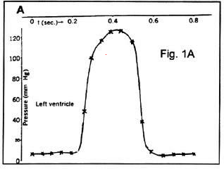
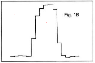
Consider the signal shown in the figure above, which is a blood-pressure signal
from the left ventricle of the heart. It is an analog signal, since it is continuously changing in time. The object of A/D conversion is
to convert this analogue signal into a digital representation. A digital
signal is a sampled signal: it is obtained by sampling the analogue
signal at discrete points in time. These instants are usually evenly
spaced in time, with the time between points being referred to as the
sampling interval.
Figure 1B shows an analog representation with digital samples taken at 0.05sec intervals as indicated at bu the x's. Each sample has a discrete value and the digital representation Fig1B is a good (albeit inexact) representation of the analog signal. You can thinks of the digitized signal as being held constant
in the time between samples.
You will use an open source program, Audacity ![]() , to generate audio signals over a wide range of frequencies and intensities. It has been installed an can be found on the doc of the SH217 Macs. Audacity is a powerful tool for creating and editing audio files. Learning to manipulate Audacity is not central to Comp Phys so in order to save time, I have used it to create a series of sound files that you can play back for digital analysis. If you enjoy manipulate audio files (converting analog vinyl to digital CD's for example it can be useful and You can download a copy for your computer (free) at Sound forge.
, to generate audio signals over a wide range of frequencies and intensities. It has been installed an can be found on the doc of the SH217 Macs. Audacity is a powerful tool for creating and editing audio files. Learning to manipulate Audacity is not central to Comp Phys so in order to save time, I have used it to create a series of sound files that you can play back for digital analysis. If you enjoy manipulate audio files (converting analog vinyl to digital CD's for example it can be useful and You can download a copy for your computer (free) at Sound forge.
It is important to remember that the computer and its speakers will limit the range of frequencies available. While human hearing is usually between 20Hz and 20KHz The Mac will limit the output. It wont go below 100 Hz or above 10KHz.
Set up the MP35 hardware  Click for the entire manual
Set up the sine wave input:
MP35 settings Click for the entire manual 
The MP35 needs a lot of information about what to expect and how you want the data to be processed. It needs to know how much you want it amplified, if AC or DC coupling is required, what filters you want to use, How you want the input and output values mapped, What units you will be using, How you want the data recorded and stored, how often you want to sample the data along with lots of other stuff. Fortunately, this can (and usually will be) preprogrammed into a template file. This can be preloaded and save a lot of valuable lab time. We will start out preprogrammed and simply make some minor changes as we go. As the semester progresses you will be involved in more setup manipulations.
Load the template
Saving your data
Set up the sine wave generator
Clean up the appearance of the graph


Some analysis of the data


You can review your data and perform analysis outside of this lab by downloading the free analysis program. Go to BSL Analysis and download the version compatible with your computer. This will allow you to work at home on data files collected in the lab.
The computer's Analog/Digital converter (ADC) allows an electrical signal to be sampled and converted into a digital signal, which is then sent within the computer for further processing. An ADC samples the analogue voltage at its input at a point in time and converts it into a 12-digit binary number. Since each digit of a binary number can take one of the two values 0 or 1, a 12-bit (bit = binary digit) number can take one of 2^12 = 4096 values, representing the integers from 0 to 4095. This integer number is then sent to the computer. The MP35 converts voltages over a range of ±10volts (a 20 volt range). In this case the A/D conversion of +10 and -10 volts would be:
| With no amplification (gain=1) | With amplification (gain =10) | |||
| Voltage | -10V | +10V | 1V | -1V |
| Binary value | 000000000000 | 111111111111 | 000000000000 | 111111111111 |
| Decimal value sent to the computer | 0 | 4095 | 0 | 4095 |
The input voltage range within -10 to +10 volts is divided into 4096 levels (the integers values 0 - 4095), with each level being 20volts/4096 = 0.0049 volts wide. An input voltage lying within one of these 4.9 millivolt-wide ranges is converted into a specific binary number: for example, any voltage lying in the range from -10.0000 to -9.9951 will be converted into the binary number 000000000000, while any voltage in the range between 9.9951 and 10.0000 volts will be converted into the binary number 111111111111, which is equivalent to the decimal number 4095. It is important to keep the input signal within the input voltage range of the ADC. If the input voltage exceeds the ±10 volt range, a 12-bit binary number with an equivalent decimal value of 4095 is still returned to the computer. The computer would thus interpret this voltage as +10 volts, which would be in error. This error is called saturation of the ADC. However, the input signal to the ADC should also span as much of the ADC input voltage range as possible, without saturating the ADC, since this increases the signal and decreases noise.
.jpg) For
example, if the signal to be recorded is much smaller than ±10
volts, say ±1 volts, it could first be amplified by a factor
of 10 (gain=10) and then sent to the converter. Note that computer
is now sent a value of 0 for -1V and a value of 4095 for an input of
+1V. These are exactly the same decimal values that were sent for
+10 and -10V. The computer and the graphing software can not tell
the difference unless you provide them with map values. You tell
it that 10V in to the converter maps to a value of 1Vinto the amplifier
(with a gain of 10) it will display real values on the graphs. This
also decreases the operating range of the data acquisition because all
voltages lower than -1V will send a value of 0 to the computer and all
voltages greater than +1V will send a value of 4095. The amplifier
allows the experimenter to record the ±1 volt signal with a significant
improvement in signal resolution (10 times greater). This occurs because,
at a gain of 10 the minimum resolvable voltage would be 1volts/4096
or 0.00049 volts versus 0.0049 volts with out amplification.
For
example, if the signal to be recorded is much smaller than ±10
volts, say ±1 volts, it could first be amplified by a factor
of 10 (gain=10) and then sent to the converter. Note that computer
is now sent a value of 0 for -1V and a value of 4095 for an input of
+1V. These are exactly the same decimal values that were sent for
+10 and -10V. The computer and the graphing software can not tell
the difference unless you provide them with map values. You tell
it that 10V in to the converter maps to a value of 1Vinto the amplifier
(with a gain of 10) it will display real values on the graphs. This
also decreases the operating range of the data acquisition because all
voltages lower than -1V will send a value of 0 to the computer and all
voltages greater than +1V will send a value of 4095. The amplifier
allows the experimenter to record the ±1 volt signal with a significant
improvement in signal resolution (10 times greater). This occurs because,
at a gain of 10 the minimum resolvable voltage would be 1volts/4096
or 0.00049 volts versus 0.0049 volts with out amplification.
Remember that you input the sine wave signal not directly into the A/D converter but into an amplifier with a gain of 10. This amplification increased the input signal voltage by a factor of ten before delivering it to the A/D converter. You informed the computer of this by selecting the gain. This version of the software will map input to output voltage values automatically. We will discuss transducer mapping later.
Now lets examine the effect of gain on acquisition.
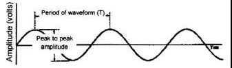
The sampling rate is the frequency at which the ADC samples the analogue signal. Generally speaking, the faster the rate at which a signal changes, the higher the frequency content of the signal, and the higher is the sampling rate needed to reproduce it faithfully. In fact, it can be proven mathematically that the sampling rate must be greater than twice the highest frequency contained in the analogue signal. This critical sampling rate is called the Nyquist Sampling Rate.
In statistics, signal processing, computer graphics and related disciplines, aliasing refers to an effect that causes different continuous signals to become indistinguishable (or aliases of one another) when sampled. It also refers to the distortion or artifact that results when a signal is sampled and reconstructed as an alias of the original signal.
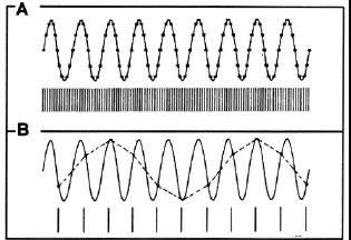
In the figure A above, the times at which A/D conversions are made are given by the vertical lines beneath the signal, while the asterisks on the wave form show the voltages that are sampled. The highest frequency present in this signal is the frequency of the signal itself, since it is a simple sine wave and thus contains only one frequency. Note that the sampling rate here is about ten times higher than the highest frequency present in the signal, and so is about five times the Nyquist rate. The sampled signal, represented by the sequence of asterisks, is thus a reasonable approximation to the analogue signal. Fig. B shows the situation that results when the sampling rate is reduced to about 1.2 times the highest frequency contained in the analogue signal. This sampling rate is thus lower than the Nyquist rate, and the sampled signal (dashed line) bears little resemblance to the analogue signal. Note that the frequency of the sampled signal is much smaller than that of the analogue signal. This artifact result due to improper choice of the sampling rate is called aliasing.
It should be clear that sampling faster is better. So why not put the peddle to the metal and leave it there?
For example, in experiments in which the resting membrane potential of muscle is measured, a sampling rate of about 20-50 Hz is sufficiently high. In contrast, when measuring action potentials in nerve axons, which are much more rapidly changing events, a sampling rate of 10-50 kHz is require. Biological signals acquisition sampling rates beyond a certain point do not significantly increase the fidelity with which the signal is rendered. In addition, increasing the sampling rate could require excessive amounts of computer processing time and storage space. Consider a semester long ecology project in which you need to record temperature, salinity, turbidity, nitrate and phosphate levels. This would require in excess of 500Tb of disk space or about $250,000 worth of hard drive. Now think about how long it would take to load the file for analysis on a WinDoz machine. The bottom line is the lower limit for sampling frequency is established by the data - the upper limit by practicality. Sampling rates beyond a certain point do not significantly increase the fidelity with which the signal is rendered.
Noise Reduction
Physiological signals recorded during experiments often contain noise at frequencies higher than those in the signal of interest. To deal with this problem, the signal is passed through a low-pass filter before sending it on to the ADC. This filter acts to remove the high-frequency noise content of the signal that would otherwise alias down in frequency when digitized, and produce spurious low-frequency content (as shown in Fig. B above). However, if the signal contains high frequency information of physiological importance, 'anti-alias filtering' would also remove components of the physiological signal. Therefore, if it is important to retain these higher frequencies, one has no choice but to use a high sampling rate when acquiring data
What does aliasing and sampling frequency have to do with real signals.
When recording from biological systems, it is common to have high frequency e.g. 5000 Hz noise. What is the frequency of an action potential?
If we sample biological data at a low frequency, high frequency noise can cause aliasing artifacts. In order to work around this we can employ an anti-aliasing or low pas filter to remove frequencies above those of interest.
The significance of Gain, sampling frequency, and aliasing to interpreting your data should now be a bit more clear.
Your data analysis quiz
You will not be asked to set up a lab experiment (except independent prophets) on your own. It takes up too much lab time. That said, you should still be able to do it. You should be able to establish sampling frequencies, gain settings and the length of an acquisition window. You should understand the problems of aliasing well enough to prevent aliasing interference with your acquisition. Go ahead and try one on your own.
September 8, 2014
Walter I. Hatch
wihatch@smcm.edu
September 8, 2014

